频率-温度叠加主曲线的构建
简介
高频测试需求
如今,许多材料都承受着反复的机械力或应力作用。例如:涡轮系统中的某些聚合物连接部件,或轮胎表面反复接触路面。为表征材料在这种作用下的表现,DMA是最有效的工具之一。
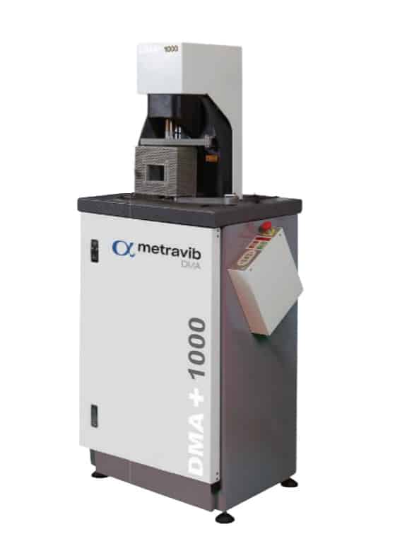
Alpha Metravib DMA+能够在高力值范围、高位移以及高达1000 Hz的高频率条件下对试样进行研究。虽然1000 Hz的频率范围已覆盖聚合物材料的绝大多数直接应用场景,但在更高频率下研究材料的粘弹性特性,仍能在特定情况下提供有关材料行为的关键信息。
一个典型的例子是评估轮胎或鞋底在特定平坦路面上的抓地性能。在这类情况下,1000 Hz以上的粘弹性特性是预测汽车(或跑者,在鞋类应用中)在这些路面上表现的关键特征。
遗憾的是,由于机械结构的限制,常规DMA仪器无法在1000 Hz以上进行测试。
FREE DOWNLOAD
Introduction to Dynamic Mechanical Analysis for Rubber Materials
主曲线原理
为克服这一限制,可采用FTS(频率-时间叠加)方法,基于WLF模型(Williams-Landel-Ferry方程)或Arrhenius模型构建主曲线。
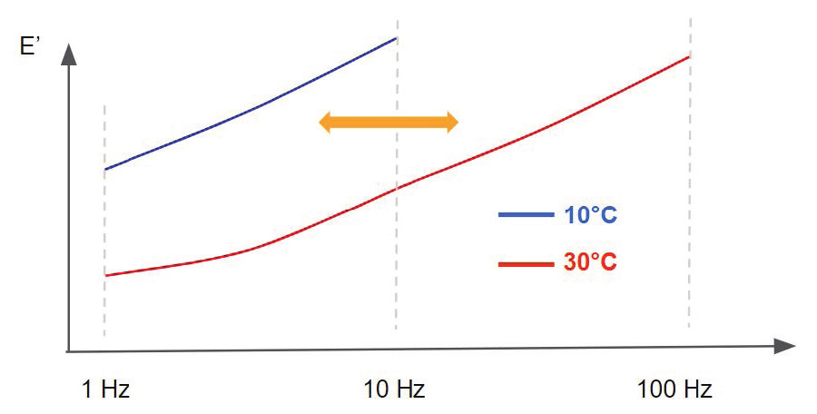
该原理十分简单:材料粘弹性特性中,机械激励的频率与温度之间存在等效关系。图2以10°C和30°C下、频率范围为1 Hz至100 Hz的两条虚拟频率扫描曲线为例,展示了这一原理——弹性模量在10°C下1 Hz至10 Hz区间内的数值,与30°C下10 Hz至100 Hz区间内的数值相同。
从分子层面看,当施加变形或力时,聚合物链会表现出相似的行为,而这种行为同时取决于温度和频率。例如,当聚合物承受恒定载荷时,E’会随时间下降,因为聚合物链会重新排列以降低所施加的应力。这也解释了为何弹性模量在低频下较低。
另一方面,升高温度(相当于向体系提供能量)会加速聚合物链在受到机械激励时的运动与重排。由此可见,降低频率对粘弹性特性产生的影响与升高温度类似。当然,反之亦然:提高频率相当于降低温度。
换言之,在DMA测试中提高试样所受机械激励的频率,对E’、E”和Tan δ产生的影响,与降低温度相同。
Alpha Metravib的DMA+仪器可在最高1000 Hz的频率下进行测试,温度范围为−150°C至500°C。基于这些技术规格,若要研究材料在1000 Hz以上的粘弹性特性,需要在不同温度下进行频率扫描,并利用频率-温度等效关系来模拟极高和极低的频率。
预备测试
在进一步设置参数之前,构建主曲线前需要考虑两个非常重要的要点(在某种程度上也可视为规则)。
第一点是必须始终处于材料的线性区域内。需要提醒的是,线性区域对应的应变幅值范围内,粘弹性特性不会随应变而改变。换言之,测试中施加的力必须足够小,以避免在聚合物基体中引发较大的分子重排。
从技术角度而言,为满足这一要求,需要在构建主曲线之前先进行应变扫描(结果部分给出了相关示例,见图5),以确定线性区域。
第二点是确定粘弹性特性随温度变化的分布情况。如前所述,主曲线是通过整合在不同温度下进行的频率扫描而构建的。若数据不足,主曲线的构建将更加困难,且很可能不完整。
因此,从最低温度到最高温度,需要考虑粘弹性特性在每个温度步长之间的变化程度,并据此设置参数。尤其是在玻璃化转变过程中,E’、E”和Tan δ会发生显著变化,因此在该转变区域内增加频率扫描的次数十分重要。
因此,强烈建议在构建主曲线之前先进行温度扫描,以确定玻璃化转变的温度范围。与上述第一点相同,结果部分也给出了相关示例(见图6)。
WLF定律适用于高于Tg的参考温度:Tg < 参考温度 < Tg + 100°C
FREE DOWNLOAD
Introduction to Dynamic Mechanical Analysis for Rubber Materials
主曲线的构建
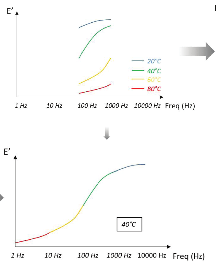
Technically, the first step in building a master curve is to perform successive frequency sweep tests at different stabilized temperatures (details are given in the Methods section). The frequency sweeps are then horizontally shifted toward a reference temperature, usually corresponding to one of the frequency sweep curves performed.
Vertical shifting of the curves is also possible when building a master curve; however, this approach is not discussed in this article. Figure 3 illustrates the process used to construct a complete master curve.
This process can be performed automatically using the Dyna+ software, or manually using a spreadsheet program.
WLF Model
The degree of horizontal shifting required to align the frequency sweeps with the reference curve can be determined as a function of temperature. Generally, two models are used to build the master curve.
The Williams–Landel–Ferry (WLF) relation, based on the principle of time–temperature superposition, is the most commonly used model. It is particularly well suited for temperatures close to the glass transition temperature and is favored for its flexibility. The WLF model describes the variation of the shift factor with temperature, as shown below.
WLF Model: log(aₜ) = − C₁(T − T₀) / [C₂ + (T − T₀)]
In this formulation, aₜ is the shift factor, T is the temperature, T₀ is the reference temperature, and C₁ and C₂ are two positive constants that depend on the material and the chosen reference temperature.
In other words, determining C₁ and C₂ allows the shift factor to be calculated (see Figure 8 in the Results section). Once the shift factor is known, any curve measured at temperature T can be shifted relative to the reference curve at T₀.
Arrhenius Model
The other model used to determine shift factors as a function of temperature is the Arrhenius model. The relationship between the shift factor and temperature can be described using the equation shown below.
Arrhenius Model: log(aₜ) = − (Eₐ / 2.303R) × (1/T − 1/T₀)
In this formulation, Eₐ is the activation energy, R is the universal gas constant (8.31 J·mol⁻¹·K⁻¹), T is the temperature, and T₀ is the reference temperature.
The Arrhenius law is well suited to describing polymer behavior below the glass transition temperature and applies effectively to secondary transitions. It is also useful for determining the activation energy associated with the glass transition.
FREE DOWNLOAD
Introduction to Dynamic Mechanical Analysis for Rubber Materials
Materials & Methods
Specimens
Rubber materials were studied using a DMA+1000 in film shear mode. A rubber film was prepared with the following dimensions:
- Length: 50 mm
- Width: 11.27 mm
- Thickness: 2 mm
Methods
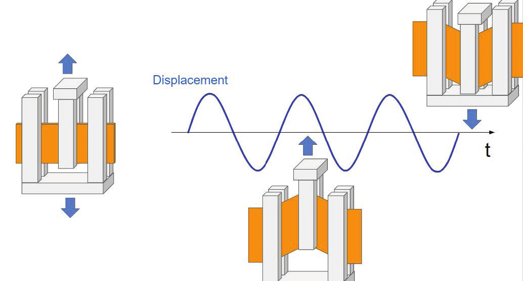
A sinusoidal waveform is applied to the specimen at different frequencies (see Figure 4) and at different temperatures. To study the specimens, the shear film mode was used.
A dynamic displacement is applied to the specimen, and shear is applied to the two parts of the specimen between the specimen holder jaws. One of the advantages of this method is that no static load is necessary to maintain the specimen in the specimen holder.
The specimen must have a form factor that complies with the dimensioning rules for the excitation mode and must exhibit a stiffness variation range compatible with the instrument’s measurable stiffness range.
Moreover, it is important to use a homogeneous (no copolymers), isotropic, and amorphous specimen, and to ensure that no structural changes occur over the characterization temperature range (e.g., post-firing or decomposition).
The following tables show the different parameters used for the two preliminary tests and for the Master Curve itself.
Table 1. Strain Sweep Setting Parameters
| Dynamic | Force from 0.01 to 50 N |
|---|---|
| Frequency | 1 Hz |
| Static | — |
| Temperature | Room temperature |
Table 2. Temperature Sweep Setting Parameters
| Dynamic displacement | 5 µm |
|---|---|
| Frequency | 1 Hz |
| Static load | — |
| Temperature | From −100°C to 80°C, at 2°C/min |
Table 3. Frequency Sweep / Master Curve Setting Parameters
| Dynamic displacement | 5 µm |
|---|---|
| Frequency | From 1 Hz to 100 Hz |
| Static load | — |
| Temperature | 15 minutes stabilization at −75°C, followed by a frequency sweep. The process is repeated at −70°C, −65°C, −60°C, −55°C, −50°C, −45°C, −40°C, −35°C, −30°C, −25°C, −20°C, −15°C, −10°C, −5°C, 0°C, and 10°C. |
Results
Preliminary Strain Sweep Results
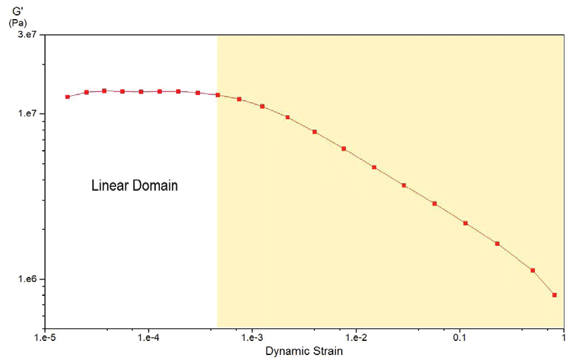
Figure 5 shows the modulus of elasticity G′ and Tan δ as a function of displacement at 1 Hz and room temperature. The graph clearly shows that the linearity domain is obtained for strain values below 0.05% (which corresponds to a 5 µm displacement). Above this range, the modulus decreases, and these changes are correlated with the nonlinear domain.
To build a proper master curve, the experiment must be performed within the linearity domain; otherwise, the curve superpositions are meaningless.
Preliminary Temperature Sweep Results
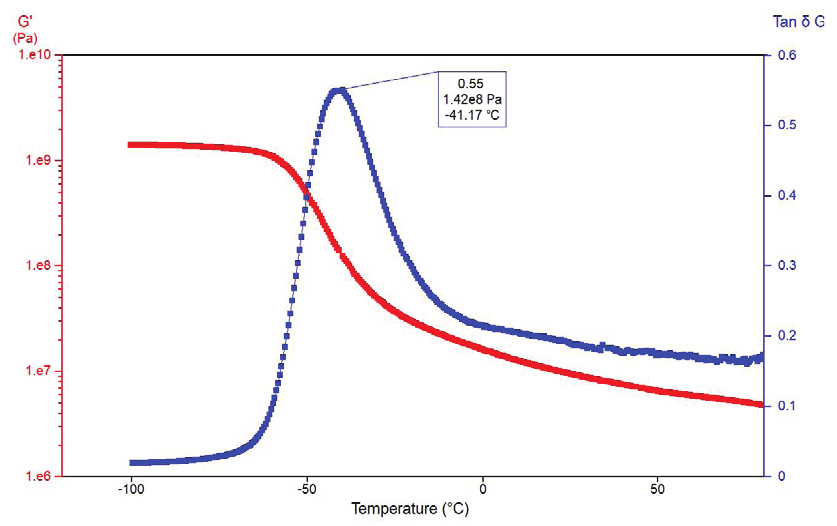
Figure 6 presents G’ and Tan δ as a function of temperature. The decrease in modulus with increasing temperature and the tan δ peak at −41.17°C are characteristic of a glass transition in the rubber.
During this transition, a gradual and reversible change occurs in amorphous materials, from a hard and relatively brittle “glassy” state to a viscous or rubbery state as the temperature increases.
This information is important for setting up the master curve experiment, because more data are required around the glass transition temperature. In other words, additional frequency sweeps must be performed near the glass transition temperature in order to obtain sufficient data to construct the master curve.
Building the Master Curve
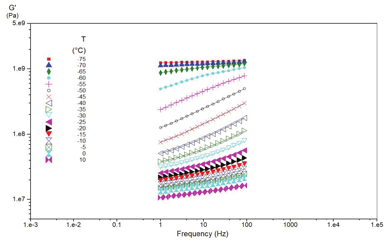
From the results obtained, frequency sweeps were performed between −75°C and 10°C, and from 1 Hz to 100 Hz at each temperature step. Figure 7 shows E′ as a function of frequency at different temperature steps; each curve can be shifted in order to build a master curve. As expected, the modulus increases slightly with frequency and decreases with temperature.
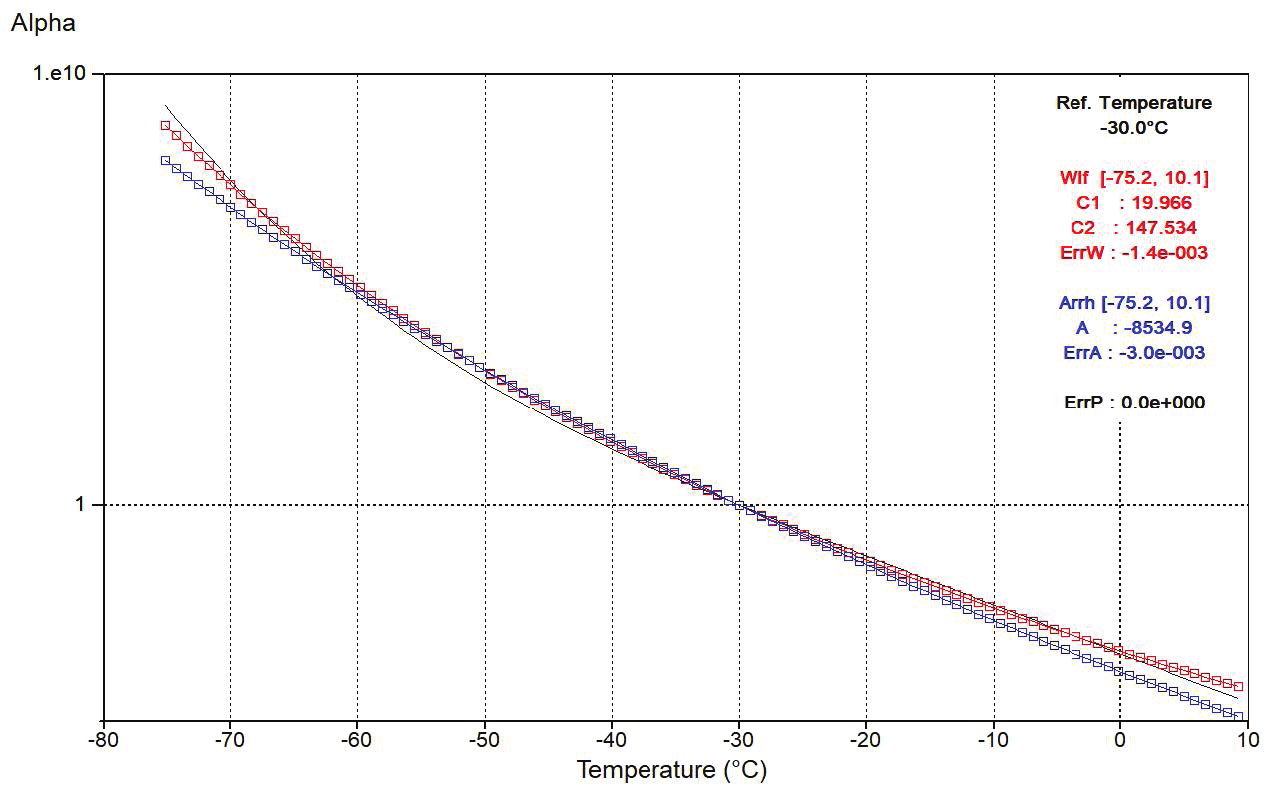
The computation performed by the DMA+ software allows the shift factor to be obtained as a function of temperature (Figure 8, with −30°C as the reference temperature). A shift factor of 1 means that there is no shift at this temperature, which is expected since −30°C is the reference.
The further the shift factor deviates from 1, the more significant the shift. As shown in the graph, both the WLF and Arrhenius models are used to fit the results (see equations in the previous section). The values C₁ and C₂ for the WLF model and A for the Arrhenius model are not provided merely for information, but primarily to allow the user to reconstruct the master curve using a spreadsheet program.
Because the error between Arrhenius and the WLF model is in favor of the WLF model (see Figure 8), the fit is based on the empirical relationship of Williams-Landel-Ferry (WLF Model), with the following parameters obtained from the DMA+ software:
- C1 = 19.966
- C2 = 147.534
- Error = 2 × 10⁻³
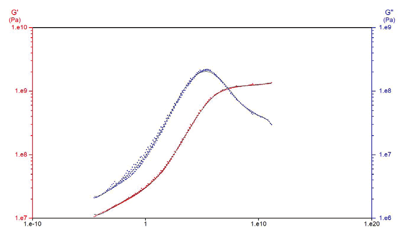
Figure 9 shows the master curve built from the combination of all frequency sweeps (Figure 7), shifted using the aₜ values shown in Figure 8. Figure 9 presents the extrapolated viscoelastic properties G′ (red squares), G’’ (blue squares), and the polynomial fit (black line) as a function of frequency.
The variations in G′ and G’’ as a function of frequency are similar to those observed during a temperature sweep (see the Preliminary Tests section), and G’’ is correlated with relaxation times. Moreover, these results highlight the capability of the master curve to predict material properties over a wide frequency range (in this example, from 10⁻⁵ to 10¹⁰ Hz).
In Figure 9, all curve shifting was performed automatically using the Dyna+ software from Metravib Material Testing.
Conclusions
KEY TAKEAWAY
Frequency–temperature superposition enables prediction of viscoelastic behavior over frequency ranges beyond direct DMA measurement.
LEARN MORE ABOUT DMA
Introduction to Dynamic Mechanical Analysis for Rubber Materials
How rubber engineers evaluate real world material behavior
Inside the guide: guidance for improving analysis quality and useful direction for integrating DMA into research, development, and testing workflows.